How to read this study
| Known from the project account | Local channel/gusset reinforcement; existing footprint and interfaces retained. |
|---|---|
| Assumed for the worked example | 150 mm effective strip, 600 mm span, 1000 N load and ideal composite action. |
| Check on the reasoning | Equilibrium, section properties and weld shear-flow check. |
| Still to verify | Real load distribution, weld design, dynamic response and recorded alignment values. |
A stable shaft line begins below the machine.
The pump base frame had a fabrication problem: weld distortion reduced mounting-pad flatness and moved the pump and motor out of alignment. Replacing the entire baseplate would affect cost and production. The existing footprint, jigs and equipment interfaces had to remain.
I measured the frame against the drawing, compared a heavier plate with local reinforcement, and selected channel stiffeners and gussets beneath the mounting zones using available shop stock. A fabrication review led to short, balanced, staggered weld runs. The model was also checked for bolt access, coupling-guard removal and maintenance clearances. Post-weld flatness and alignment checks were required.
The project account reports that the reinforced frame met its alignment target without replacing the baseplate. It does not provide dimensions, numerical readings or the acceptance tolerance. The geometry and numbers below form a worked teaching example of the same design decision.
If one foot is high, tightening it to the floor bends the table. If the tabletop is flexible, it can still sag after all four feet touch. A pump base has the same two problems: initial geometry and loaded stiffness. Correcting one does not automatically correct the other.
1. A small foot-height difference becomes a shaft-angle error.
Imagine the front and rear motor-foot stations are 400 mm apart. Relative to the desired cold shaft line, the front is 0.20 mm high and the rear is 0.08 mm high. For a rigid motor with equal transverse foot heights, the slope comes directly from a right triangle:
θ = atan[(0.08 − 0.20)/400]
θ ≈ −0.000300 rad = −0.0172°
The minus sign means the motor axis falls toward the rear. If the coupling is 150 mm in front of the front-foot station, extrapolate the same straight line:
y(−150) = 0.20 + (−150)(−0.12/400)
Coupling-plane offset = 0.245 mm high
The coupling can therefore see both offset and angular error. Moving the motor by one uniform shim thickness changes offset but leaves the slope unchanged. Under the assumed geometry, lowering the front by 0.20 mm and the rear by 0.08 mm restores the target line. That is only possible by removing available shims or correcting the mounting geometry—not by forcing the feet down with bolts.
This is a two-dimensional geometry example, not a field alignment prescription. Actual correction requires horizontal readings, soft-foot checks, shaft geometry, machine restraints and the manufacturer's cold alignment target. Three-dimensional twist cannot be diagnosed from two heights.
2. Separate flatness, soft foot and elastic deflection.
Flatness describes the geometry of a surface. A collection of individually flat pads can still lie at different heights; the drawing must state the intended common mounting plane. A range of dial readings relative to one setup plane is not automatically a formal minimum-zone flatness measurement.
Soft foot means the machine is not supported consistently at its feet. Gaps, tilted pads, burrs, damaged feet or poor shim contact can make bolt tightening distort the machine. A flat base alone does not guarantee a soft-foot-free machine.
Elastic deflection is movement under load. A frame can be flat while unloaded yet bend after equipment, pipe loads and bolt preload are applied. Reinforcement helps this stiffness problem, but it does not by itself straighten an already distorted pad.
Weld metal and the heated surrounding material expand and contract unevenly. Restraint and non-uniform cooling can leave residual stress and permanent deformation. The simple elastic relation ε = αΔT explains free thermal strain; it cannot predict final weld distortion once restraint, plasticity and transient temperature fields matter. TWI describes these mechanisms and the role of weld arrangement in its distortion guidance.
3. Inspect the proposed load path in 3D.
The study retains a 1200 × 600 mm footprint and a 10 mm baseplate. Two idealized 80 × 40 × 6 mm channels sit below the mounting zones. Four pads are 120 × 100 × 12 mm, with eight Ø18 mounting holes. Local 6 mm gussets connect the pad region to the channel web.
Loading the CAD model…
Blue: retained baseplate · Green: channels and gussets · Grey: pads and idealized supports. Rotate underneath to see the reinforcement.
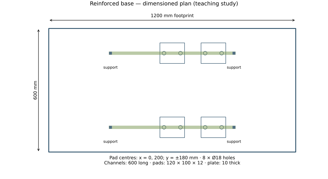
The support centres define a 600 mm analytical span. The blocks represent boundary conditions, not a designed foundation. Weld beads, actual stock corner radii, anchor bolts and machine bodies are omitted. Production drawings must specify welds, machining allowances, fits and inspection requirements.
4. Reduce the problem to a reviewable beam model.
Consider one 150 mm-wide effective strip of the mounting zone carrying a central 1000 N vertical load over a simply supported 600 mm span. Take E = 200,000 N/mm² for the steel stiffness calculation. Use the same span and load for all three options:
- A retained 10 mm plate strip.
- A 20 mm plate strip.
- The 10 mm strip acting compositely with an 80 × 40 × 6 mm idealized channel.
The strip width is an assumption, not a measured effective width. The beam calculation excludes the gussets and pad thickness. It assumes small deformation, elastic material response and complete shear transfer between plate and channel. It does not model plate bending in two directions, channel torsion, bolt preload or the full machine load distribution.
Why use it? It isolates the design choice: add material everywhere, or place it farther from the neutral axis directly beneath the load path. A detailed plate or finite-element model can then test whether the simplified load path is credible.
5. Where the bending formulas come from.
Start with three ideas: plane sections remain plane, elastic stress is proportional to strain, and internal forces balance the applied moment. A fibre a distance y from the neutral axis has strain ε = κy, where κ is curvature. Hooke's law gives σ = Eκy. Sum the moment of stress over the section:
Define I = ∫y² dA → M = EIκ
Therefore σ = My/I
I is the second moment of area, measured in mm⁴. Material farther from the neutral axis contributes in proportion to distance squared. For a rectangular section, integrating horizontal strips gives:
For the retained strip, I = 150 × 10³/12 = 12,500 mm⁴. Doubling thickness gives I = 150 × 20³/12 = 100,000 mm⁴: eight times the bending stiffness, not twice. The geometric and material foundations are also developed in Cambridge's beam-curvature explanation.
Derive the central-load deflection.
Symmetry and vertical force balance give each support a reaction P/2. On the left half of the beam, at distance x from its support, M(x) = Px/2. For small slopes, curvature is approximately the second derivative of vertical displacement, v″.
EI v′ = Px²/4 + C₁
EI v = Px³/12 + C₁x + C₂
At x = 0, the support displacement is zero, so C₂ = 0. At midspan x = L/2, symmetry makes the slope zero, giving C₁ = −PL²/16. Substitute x = L/2 into the displacement expression:
Downward deflection magnitude: δ = PL³/(48EI)
The factor 48 comes from this load case and these boundary conditions. It must not be carried over to a cantilever, a distributed load or a different support arrangement.
6. Put the added steel where it creates leverage.
The plate and channel share one neutral axis only if their connection transfers longitudinal shear. Measure vertical coordinates from the underside of the plate: the plate lies from z = 0 to +10 mm and the channel extends to −80 mm.
Divide the section into non-overlapping rectangles: plate 150 × 10 at z = +5; web 6 × 68 at z = −40; top flange 40 × 6 at z = −3; bottom flange 40 × 6 at z = −77 mm. The web excludes the flange thickness to avoid double counting.
z̄ = ΣAᵢzᵢ / ΣAᵢ = −11.7337 mm
The parallel-axis theorem follows by expanding ∫(y+d)²dA about each rectangle's centroid. Its first moment ∫y dA is zero, leaving I = Icentroid + Ad². Apply it to all four rectangles:
I = 1,957,799 mm⁴
This ideal composite strip has about 156.6 times the I of the 10 mm strip. It is a theoretical sectional comparison, not a claim that the entire fabricated frame becomes 156.6 times stiffer.
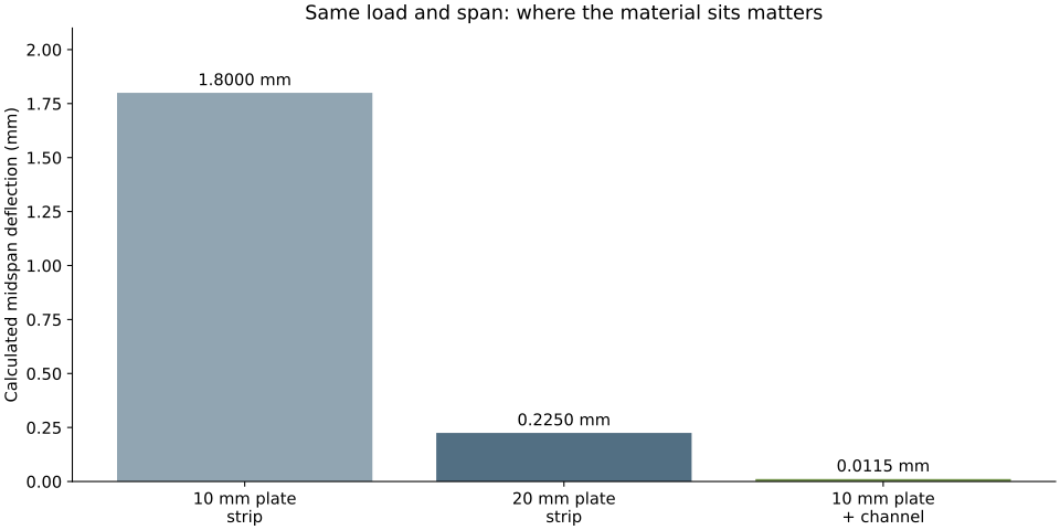
δ20 mm = 0.225 mm
δplate + channel = 0.01149 mm
All three values use P = 1000 N, L = 600 mm and E = 200,000 N/mm². For a teaching screening limit of 0.05 mm, only the composite option meets this particular simplified check. The 0.05 mm limit is not the original project's alignment tolerance and is not a universal acceptance criterion.
Check stress as well as stiffness.
The maximum moment is PL/4 = 150,000 N·mm. The 10 mm strip has maximum bending stress 150,000 × 5/12,500 = 60.0 MPa. For the composite, the extreme bottom fibre is 68.2663 mm from the neutral axis, giving 5.23 MPa. These elastic nominal stresses exclude weld toes, bolt holes and other stress concentrations. A low nominal stress does not establish fatigue life or a factor of safety without a specified material and load spectrum.
7. The weld connection makes composite action possible.
The plate's share of bending stress changes along the span as the moment changes. The connection must transfer that changing longitudinal force into the channel. From the bending stress distribution, the required interface shear flow is:
QA = Aplate(zplate − z̄)
QA = 1500(5 + 11.7337) = 25,100.5 mm³
V = P/2 = 500 N
q ≈ 6.41 N/mm
QA is the first moment of area above the interface, not fluid flow. One way to derive q is to integrate σ = My/I over the plate to obtain its longitudinal force N = MQA/I, then differentiate along the beam: dN/dx = (dM/dx)QA/I = VQA/I.
This is the total longitudinal transfer demand per unit length in the ideal beam. Distribution between weld lines depends on their arrangement. It is not a weld-size specification: start/stop effects, eccentric loads, fatigue, local peel, weld strength and connection stiffness still require review. Intermittent welds also concentrate transfer into their welded lengths.
The gussets shorten local load paths beneath the pads and help resist local rotation, but their benefit is not credited in the beam calculation. Avoid creating a stiff point beside an unsupported flexible plate region. Check bolt and tool access before finalizing their position.
8. Add stiffness without adding a new distortion problem.
More weld metal can mean more shrinkage. The fabrication plan must therefore accompany the reinforcement design. The project used short, balanced, staggered runs after shop review, rather than allowing distortion to accumulate unchecked on one side.
A practical sequence establishes the drawing datum and jig condition, fits and tacks the reinforcement, checks the mounting geometry, then follows the approved weld sequence and rechecks after cooling and release from restraint. The specific run lengths, preheat, interpass controls and weld sizes belong in the reviewed procedure; they cannot be selected from the static beam calculation.
TWI discusses balanced welding and skip/back-step techniques in its fabrication guidance. Restraint can limit movement while welding but does not prove the released assembly will remain flat. Where required, plan machining allowance and a post-weld finishing operation to establish the mounting plane.
Material choice should preserve weldability, available stock, corrosion protection and suitable properties for the service temperature. A higher yield-strength grade does not materially increase stiffness if its elastic modulus is similar. The I term is doing the work in this example. Actual stock channels also have corner radii and certified section properties; use those for a release calculation.
9. Change the load and see the stiffness response.
Keep the section properties and E fixed, then vary load and span. This makes the P and L³ dependence visible. These controls change the analytical example, not the dimensioned CAD.
Doubling load doubles deflection; doubling span multiplies it by eight in this model. Improving support location can therefore be as important as increasing section stiffness. Shorter, deeper configurations may need shear-deformation effects included; this explorer retains the same Euler–Bernoulli approximation throughout.
10. Verify the geometry, then the assembled machine.
- Before rework: record support conditions, pad measurements, equipment interfaces and the observed alignment issue. Identify the datum and measurement method.
- After fabrication and cooling: inspect welds and remeasure the unrestrained geometry in the defined support condition. Confirm hole locations and maintenance clearances.
- Under equipment load: compare pad movement with the analysis. Check whether the actual load distribution and foundation match the assumed boundary conditions.
- At assembly: check contact and soft foot, then measure horizontal and vertical shaft alignment using the equipment procedure. Record the shim arrangement and tightening sequence.
- After final connections: repeat checks as required after anchoring, grouting or pipe connection so imposed strain is not overlooked. Use the manufacturer's operating-temperature target and vibration criteria.
A dynamic assessment may also be needed: stiffness changes natural frequencies, and a static deflection result does not prove separation from running-speed or excitation frequencies. The full frame has coupled bending and torsional modes, machine masses and foundation compliance that this strip model does not represent.
The design preserved the production interfaces while putting reinforcement beneath the loads. Its success depended on fabrication control and measured alignment—not on the appearance of the CAD model alone.
Drawings, models and calculation data.
Continue with Shaft Redesign, Pump Performance or the engineering calculators.