Problem
The pump needed pressure before it could make pressure.
A pump delivering 60 m³/h at 30 m head was operating with limited suction margin at low tank level. Replacing the pump or changing its foundation would disturb the client’s installation. I compared those options with a simpler intervention: reduce the energy lost before the water reaches the impeller.≈ Assumed
The selected change replaced DN80 suction piping with DN100 and removed high-loss fittings. Calculated NPSH available increased from approximately 3.6 to 5.1 m. The work also included the piping interface, BOM, minimum-level cut-out and low-level commissioning checks.≈ Assumed
How much pressure can we recover upstream while retaining the pump, duty point and foundation?
Constraints
2. Separate project facts from the worked example.
The recorded project values establish the design direction. The following illustrative hydraulic model reproduces the rounded 3.6 → 5.1 m comparison; it is not a recovery of the original calculation sheet. Its resistance budgets are chosen explicitly, not inferred as measured fitting data.≈ Assumed
| Input | Value | Basis |
|---|---|---|
| Duty | 60 m³/h at 30 m head | Project value≈ Assumed |
| Suction size | DN80 → DN100 | Project change≈ Assumed |
| Velocity | Approximately 3.3 → 2.1 m/s | Project calculation≈ Assumed |
| NPSH available | Approximately 3.6 → 5.1 m | Project calculation≈ Assumed |
| Fluid | Water; ρ = 998 kg/m³ | Example assumption≈ Assumed |
| Absolute pressures | Atmosphere 101.325 kPa; vapour 2.340 kPa | Example, approximately 20°C≈ Assumed |
| Hydraulic bore | 80 → 100 mm | Example; actual bore depends on pipe schedule≈ Assumed |
| Straight pipe length / Darcy f | 6 m / 0.020 | Example assumptions≈ Assumed |
| Liquid level z | −4.5104 m | Chosen example suction lift≈ Assumed |
| Total fitting K | 2.0692 → 0.9785 | Chosen budgets; referenced to each line velocity≈ Assumed |
Assumptions and limits
≈ Assumed Values carried forward from this study, not newly measured inputs.
| Assumption | Value | Basis | Effect if wrong |
|---|---|---|---|
| Water density | 998 kg/m³ | Existing worked-example input | Changes pressure-head and recovered-pressure conversion. |
| Atmosphere / vapour pressure | 101.325 / 2.340 kPa absolute | Existing approximately 20°C example | Higher vapour pressure or lower atmospheric pressure reduces available NPSH. |
| Hydraulic bores | 80 / 100 mm | Illustrative internal diameters, not DN schedule dimensions | Smaller actual bore raises velocity and losses. |
| Pipe length / Darcy factor | 6 m / 0.020 | Existing fixed-coefficient example | Length and friction error alter the predicted loss budget. |
| Aggregate fitting K | 2.069202678 / 0.978468431 | Chosen budgets in the original calculation JSON | Higher actual resistance reduces NPSH available. |
| Liquid elevation | −4.510434937 m | Chosen example suction lift; the slider adds Δz | A 1 m lower level removes 1 m of NPSH available. |
| Equal boundary conditions | Same fluid, level, flow and atmosphere for both pipes | Comparison model | Unequal conditions invalidate attribution of all recovery to reduced loss. |
| Manufacturer margin | Not supplied | No NPSHr curve or acceptance margin in this study | Calculated availability cannot establish an acceptable operating point. |
Method
1. Cavitation begins with local pressure.
Water can form vapour when its local absolute pressure falls to the vapour pressure at its temperature. Inside a pump, pressure drops as the liquid accelerates into the impeller eye. Vapour cavities can then collapse as pressure recovers, producing noise, vibration and damage.
NPSH available is the inlet total head above vapour-pressure head. It is a property of the installation. NPSH required comes from the pump’s tested performance at the relevant flow, speed and impeller configuration. These two quantities answer different questions.
For a large, vented supply tank, apply Bernoulli from the free surface to the suction reference plane. Surface velocity is negligible; the pump reference elevation is zero:
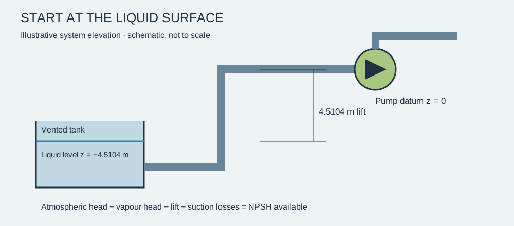
Here z is liquid-surface elevation relative to the pump: positive for flooded suction and negative for suction lift. The inlet velocity term is already included through Bernoulli; subtracting it again would double-count it.
7. Turn the pressure budget into a physical layout.
This dimensioned 2,000 mm suction-spool study includes hollow pipe bores, a full-bore valve envelope with handwheel, drilled flanges, fasteners, supports and a flat-top eccentric reducer. Blue identifies piping; green identifies the valve and reducer. It illustrates the layout decisions and does not represent the full installation’s 6 m hydraulic pipe length.≈ Assumed
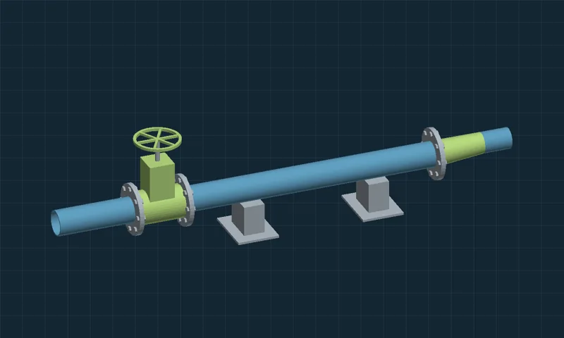
Static CAD study. Use the dimension sheet and downloads without JavaScript.
Drag or use arrow keys to rotate. Use the view buttons and zoom slider. Dimensions in mm; illustrative geometry.
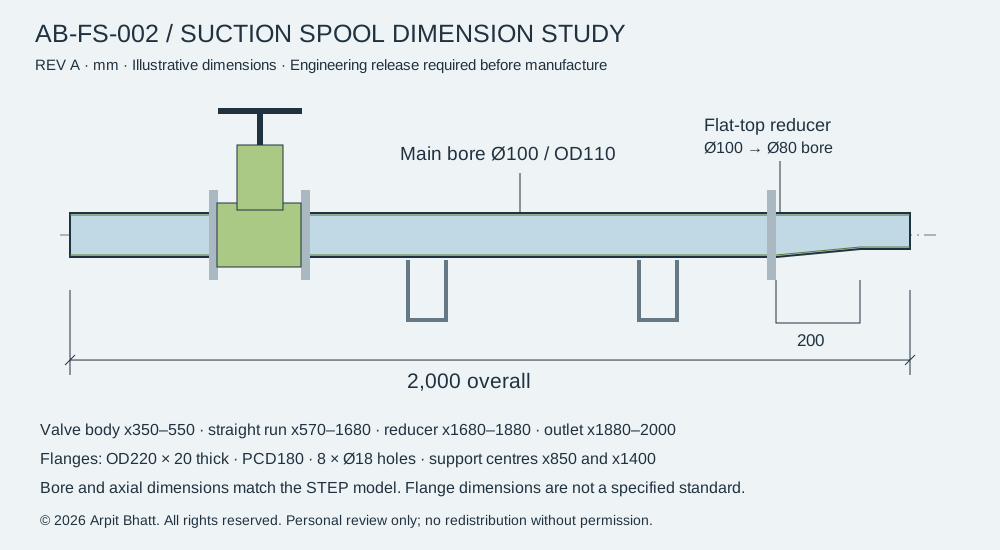
| Feature | Dimension / design intent |
|---|---|
| Overall spool envelope | 2,000 mm≈ Assumed |
| Main pipe | 100 mm ID / 110 mm OD≈ Assumed |
| Valve envelope | x = 350–550 mm; simplified full-bore passage≈ Assumed |
| Flange study | 220 mm OD; 180 mm bolt circle; 8 × Ø18 holes; 20 mm thick≈ Assumed |
| Eccentric reducer | 200 mm long; 100 → 80 mm bore; upper bore aligned≈ Assumed |
| Supports | x = 850 and 1,400 mm≈ Assumed |
| Release status | Study dimensions; flange standard, pressure rating, materials and tolerances to be specified≈ Assumed |
The reducer’s smaller centreline is raised by 10 mm to keep the upper internal surface level. A flat-top arrangement can help avoid an air pocket in a horizontal suction run; confirm orientation and straight-run requirements with the pump supplier. A reducer still creates local loss, and an undersized pump nozzle is not made larger by changing the upstream pipe.≈ Assumed
The valve and fasteners are simplified envelopes, not detailed operable internals. The model contains no asserted pressure-rating or flange-standard compliance. Its small outlet section and transitions require their own velocity-based loss treatment in a final calculation; the worked model uses aggregate resistance budgets.
Calculations
Governing equations
Continuity
Velocity equals volumetric flow divided by area; circular area equals pi times diameter squared divided by four. Formula reference →
Loss budget
Head loss equals the sum of pipe-friction and fitting-resistance factors multiplied by velocity head. Formula reference →
Available NPSH
Available NPSH equals atmospheric head above vapour pressure, plus liquid elevation, minus suction loss. Formula reference →
3. The same flow needs less velocity in a larger pipe.
A = πD² / 4 → V = Q/A
V80 = 3.316 m/s
V100 = 2.122 m/s
Increasing bore by 25% increases area by 56.25%. The velocity falls to 64% of the baseline. Because velocity head varies with V², its value falls to 40.96%—even before changing a single fitting.✓ Verified by calculation
V100²/(2g) = 0.22952 m
A nominal DN label is not an internal diameter. Before procurement, repeat this step using the selected pipe schedule and the actual restriction bores. DN100 is a comparison candidate here, not a universal suction-velocity recommendation.✓ Verified by calculation
4. Account for every metre of lost head.
The first term accounts for straight-pipe wall friction; the second accounts for local losses at entrances, valves, bends, strainers and transitions. Use the Darcy friction factor, not the Fanning factor. Each fitting coefficient must use its specified reference velocity.
| Contribution | 80 mm example | 100 mm example |
|---|---|---|
| fL/D | 1.5000 | 1.2000✓ Verified by calculation |
| ΣK | 2.0692 | 0.9785✓ Verified by calculation |
| Straight-pipe loss | 0.8405 m | 0.2754 m✓ Verified by calculation |
| Fitting loss | 1.1595 m | 0.2246 m✓ Verified by calculation |
| Total suction loss | 2.0000 m | 0.5000 m✓ Verified by calculation |
About 0.565 m of the 1.5 m recovery comes from the straight-pipe term and 0.935 m from the fitting term. Both the larger bore and lower aggregate resistance matter. The K values are illustrative totals; replace them with supplier data or defensible fitting correlations for the actual installation.✓ Verified by calculation
For a detailed check, calculate Reynolds number Re = ρVD/μ, establish roughness ε/D and obtain f from a suitable correlation or the Moody chart. This example holds f at 0.020 to expose the effect of diameter and resistance without pretending the pipe material is known.✓ Verified by calculation
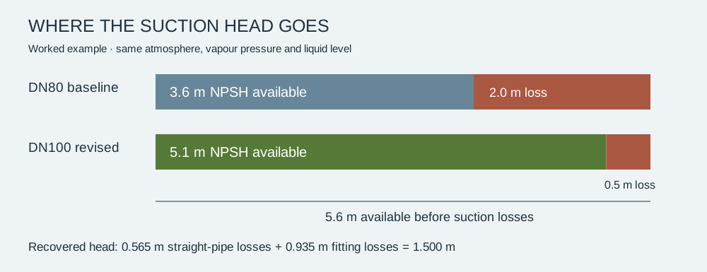
5. Recover inlet margin without changing elevation.
Head before losses = 10.1104 − 4.5104 = 5.6000 m
Baseline NPSHA = 5.6000 − 2.0000 = 3.6000 m
Revised NPSHA = 5.6000 − 0.5000 = 5.1000 m
The same atmosphere, liquid temperature and liquid level apply to both cases. The entire gain comes from reducing suction losses. The recovered 1.5 m corresponds to approximately 14.69 kPa of water pressure head.✓ Verified by calculation
The 30 m discharge duty does not belong in this NPSH equation. At the stated duty, hydraulic power is ρgQH = 4.90 kW; shaft power would require pump efficiency. Neither figure establishes the pump’s suction requirement.✓ Verified by calculation
Obtain the manufacturer’s NPSH requirement and the specified margin across the operating range. NPSH3 is associated with a 3% head drop and is not a guarantee of cavitation-free operation. No supplier NPSH curve or acceptance margin is supplied for this example.✓ Verified by calculation
6. Test what happens when conditions change.
Move the controls to inspect the same model at a different flow or tank level. Geometry, vapour pressure and Darcy f remain fixed; losses scale with Q² in this simplified sensitivity study. This is not a pump-curve simulation.
Compare the same installation at another flow
Valid input ranges: flow 30–90 m³/h; level change −1.5 to +1.5 m. These are the original educational slider ranges, not approved equipment limits. Values between slider steps may be typed.
Baseline 3.60 m · Revised 5.10 m · Recovery 1.50 m
✓ Verified by calculationArithmetic within the stated model; input assumptions apply.
Pump NPSH required and the acceptance margin are not supplied. No operating pass/fail decision is made.
Show the work: formula, substitution and result
For each pipe: QSI = Q/3600; A = πD²/4; V = QSI/A; hL = (fL/D + K)V²/(2g); NPSHA = (patm − pv)/(ρg) + z + Δz − hL.
Q = 60/3600 = 0.01666667 m³/s
H₀ = (101325 − 2340)/(998 × 9.81) − 4.510434937 = 5.6000 m
D = 0.08 m: A = 0.00502655 m²; V = 3.315728 m/s; hL = 2.0000 m; NPSHA = 3.6000 m
D = 0.10 m: A = 0.00785398 m²; V = 2.122066 m/s; hL = 0.5000 m; NPSHA = 5.1000 m
Recovery = 5.1000 − 3.6000 = 1.5000 m
Formula references: KSB head loss and KSB NPSH. Input precision: existing calculation JSON.
A 1 m drop in tank level removes 1 m of NPSH available from both cases. At 72 m³/h, losses increase by 44%: baseline NPSH becomes 2.72 m and revised NPSH becomes 4.88 m at the example level. Raising vapour pressure by 10 kPa would independently remove about 1.02 m from each result.✓ Verified by calculation
Two worked test cases
Case A: Q = 60 m³/h, Δz = 0 m. Case B: Q = 72 m³/h, Δz = 0 m. Both retain all existing inputs. Columns identify the actual hydraulic bore, not a pipe schedule.
| Formula and reference | A · 80 mm | A · 100 mm | B · 80 mm | B · 100 mm | Status |
|---|---|---|---|---|---|
| QSI = Q / 3600Unit definition: 1 hour = 3600 seconds. | 0.016667 m³/s | 0.016667 m³/s | 0.020000 m³/s | 0.020000 m³/s | ✓ Verified by calculation |
| A = πD² / 4Circle geometry. | 0.005027 m² | 0.007854 m² | 0.005027 m² | 0.007854 m² | ✓ Verified by calculation |
| V = QSI / AContinuity; KSB head loss. | 3.315728 m/s | 2.122066 m/s | 3.978874 m/s | 2.546479 m/s | ✓ Verified by calculation |
| hv = V² / (2g)Bernoulli kinetic-energy head; KSB head loss. | 0.560349 m | 0.229519 m | 0.806903 m | 0.330507 m | ✓ Verified by calculation |
| hp = (fL/D) hvDarcy–Weisbach; KSB head loss. | 0.840524 m | 0.275423 m | 1.210354 m | 0.396609 m | ✓ Verified by calculation |
| hf = K hvLocal resistance; KSB head loss. | 1.159476 m | 0.224577 m | 1.669646 m | 0.323391 m | ✓ Verified by calculation |
| hL = hp + hfSum of pipe and fitting losses. | 2.000000 m | 0.500000 m | 2.880000 m | 0.720000 m | ✓ Verified by calculation |
| NPSHA = 5.6 − hLVented-tank energy balance; KSB NPSH. | 3.600000 m | 5.100000 m | 2.720000 m | 4.880000 m | ✓ Verified by calculation |
Hand substitution · 60 m³/h
QSI = 60/3600 = 0.01666667 m³/s
H₀ = (101325−2340)/(998×9.81)−4.510434937 = 5.600000 m
D=0.08 m: A=π×0.08²/4=0.00502655 m²; V=0.01666667/0.00502655=3.315728 m/s
hL=(0.020×6/0.08+2.0692026781)×3.315728²/(2×9.81)=2.000000 m
NPSHA=5.600000−2.000000=3.600000 m
D=0.1 m: A=π×0.1²/4=0.00785398 m²; V=0.01666667/0.00785398=2.122066 m/s
hL=(0.020×6/0.1+0.9784684314)×2.122066²/(2×9.81)=0.500000 m
NPSHA=5.600000−0.500000=5.100000 m
ΔH = 5.100000−3.600000=1.500000 m
Δp = 998×9.81×1.500000/1000=14.685570 kPa
Ph = 998×9.81×(60/3600)×30/1000=4.895190 kW
✓ Verified by calculation
Hand substitution · 72 m³/h
QSI = 72/3600 = 0.02000000 m³/s
H₀ = (101325−2340)/(998×9.81)−4.510434937 = 5.600000 m
D=0.08 m: A=π×0.08²/4=0.00502655 m²; V=0.02000000/0.00502655=3.978874 m/s
hL=(0.020×6/0.08+2.0692026781)×3.978874²/(2×9.81)=2.880000 m
NPSHA=5.600000−2.880000=2.720000 m
D=0.1 m: A=π×0.1²/4=0.00785398 m²; V=0.02000000/0.00785398=2.546479 m/s
hL=(0.020×6/0.1+0.9784684314)×2.546479²/(2×9.81)=0.720000 m
NPSHA=5.600000−0.720000=4.880000 m
ΔH = 4.880000−2.720000=2.160000 m
Δp = 998×9.81×2.160000/1000=21.147221 kPa
Ph = 998×9.81×(72/3600)×30/1000=5.874228 kW
✓ Verified by calculation
Pressure recovery follows Δp = ρgΔH; hydraulic power follows Ph = ρgQH (pressure work per unit time). These are derived from pressure head and continuity. They do not provide shaft power without efficiency. The Q² check follows directly from V = Q/A at fixed geometry, f and K.
Additional exact checks: at 60 m³/h and Δz = −1 m, availability becomes 2.60 / 4.10 m; recovery stays 1.50 m. At 72 m³/h, (72/60)² = 1.44, so losses are 2.88 / 0.72 m. ✓ Verified by calculation
Reynolds-number evaluation and the minimum-level cut-out remain methods to complete, not numerical results: viscosity, manufacturer NPSH requirement, acceptance margin and sensor allowances must be established first.
Pressure/head conversion reference: KSB NPSH. Hydraulic-power reference: KSB pump power relation. The listed formulas and test cases verify arithmetic only.
Verification
8. Close the loop at the lowest operating level.
- Confirm the operating envelope. Obtain minimum tank level, maximum flow, liquid temperature range, site atmospheric pressure and the pump’s NPSH curve.
- Audit the suction path. Record actual bores, lengths, bends, valve positions, strainer clean/dirty loss and reducer geometry. Check for air ingress, vortexing and trapped-air locations.
- Set the level cut-out from a margin. Rearranging the equation gives zmin = NPSHrequired + margin + hL − (patm−pv)/(ρg). Add the appropriate allowance for sensor uncertainty and dynamic level change; no numeric setpoint is justified without those inputs.
- Commission at low level. Log flow, temperature, suction absolute pressure, discharge head, vibration and noise. Convert any gauge suction pressure to absolute pressure before evaluating NPSH.
- Review and release. Reconcile the calculation, supplier guidance, piping drawing and BOM. Record acceptance criteria and review findings.
Limits
How to read this study
| Known from the project account | Suction-system modification; reported NPSHa change from 3.6 to 5.1 m. |
|---|---|
| Assumed for the worked example | Worked losses, fluid properties and spool geometry. |
| Check on the reasoning | Energy balance and loss comparison. |
| Still to verify | Manufacturer NPSHr, margin and actual site conditions. |
Result
Worked comparison: 3.60 → 5.10 m NPSH available at 60 m³/h and unchanged level.
✓ Verified by calculationCalculation only. Final pump acceptance remains open.
The project increased calculated suction margin while retaining the required duty and client layout. The broader lesson is to treat the suction system as part of the pump design: protecting the pressure at the inlet can be more effective than changing the pump.≈ Assumed Reported project outcome; underlying site records are not supplied here.
Inspect the engineering package.
STEP is an exchange model for CAD import. Downloaded dimensions and numerical examples are illustrative; confirm the actual installation before engineering release.
Technical references
KSB: NPSH · KSB: head-loss equations. References explain the underlying theory; the project comparison and worked-example assumptions are stated above.
Sources and standards
- KSB Centrifugal Pump Lexicon: NPSH ↗ — available and required NPSH, installation boundary conditions.
- KSB Centrifugal Pump Lexicon: Head loss ↗ — continuity, pipe friction and local losses.
- Existing study calculation data — input provenance and full-precision coefficients.
- KSB Centrifugal Pump Lexicon: Pump affinity laws ↗ — defines hydraulic output power P = ρgQH; the worked cases hold duty head at 30 m and are not pump-curve predictions.
No governing pump/flange standard or edition has been established by this study. No standards compliance is claimed. The applicable project specification and manufacturer requirements remain to be supplied.
Revision history
- 3A-R1 · Case-study engine
- Reorganized existing content into seven sections. Added input validation, shareable calculation state, two worked checks, accessible equations and a print summary. Engineering inputs unchanged.
- Last reviewed
- Engineering review not recorded. Populate reviewer, date, scope and evidence only after an actual review.